WAIT TIMES FOR HIGHLY DESIRABLE WATCHES

LITTLE’S LAW

Little’s Law developed by MIT professor John Little, is a remarkably elementary but profound theorem in Queueing theory, the mathematical study of lines and queue wait times. It is predominantly used to estimate queue times in a retail business but the equation can be generalized to any stationary system, in our case, wait times for desirable watches.

We must impose ideal and somewhat unrealistic assumptions to use this model, but for our purposes it will give us a starting framework should all conditions be ideal. In a stationary system, the probability of an event happening does not vary with time.

Little’s Law states that:

L= λ∙W

where

L = the average number of items in a queueing system,

λ = the average number of items arriving in the system per unit of time,

W = the average waiting time an item spends in the queueing system,

The equality is best understood by a real life example. We will use a retail store with real people and real wait times. Let us assume an AD requires 1 salesperson to tend to a maximum 3 customers per hour to give them the optimal attention. λ is the number of persons entering the store per hour and let’s assume that the store has a maximum capacity of 40 people per hour. Assuming there is a constant influx and efflux of people per hour, we will make λ = 40 people per hour. We also assume that the average time a customer spends in the AD as half an hour, or W = 0.5 hr.

Substituting into the equality,

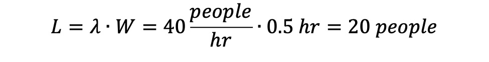
With an influx of 20 people per hour one salesperson would be inadequate to tend to all the customer’s needs and the AD would require at least 3 salespersons to work.

APPLYING TO THE WATCH SITUATION

Let us apply the above equation to our particular watch situation, a frenzy in which all watch buyers can relate to in this current and unprecedented market.

For watch buyers, we are more interested in W, the queue wait time a customer is expected to wait for their grail watch. Let us use a common and popular example these days, the Rolex Submariner date 116610LN.

Rearranging Little’s Law to:

Mathematicians of the world, please allow me to unofficially name this rewritten version as ” The Watch Equation” or please forgive me.

Remembering that:

W = the average waiting time to obtain exactly one new watch in months.

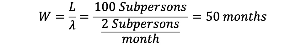
L = the average number of people waiting in the queue. This is the number that is unknown to us. But we will choose an educated and conservative guess of 100 total persons who ADs consider as eligible waitlist contenders (i.e: good credit history, genuine intention to purchase the watch etc…)

λ = the average number of watches arriving per unit of time. My AD told me they receive 2 Submariners per month on average, so for our purposes λ= 2 Subpersons/month.

We substitute into the equation:

INTERPRETATION

The end result is W = 50 months or about 4 years long, assuming that the waitlist has a constant influx and efflux of watches λ, and that the waitlist L is 100 persons long. The assumption is also that in an ideal and fair AD, distribution of watches is on a first come, first serve basis.

Of course, this may not be the case in the real world where a customer may move further up the priority list based on whatever reason the AD may decide. In this case, the customer may move up the list to 50th position and the L would change to 50 persons and their wait time would be cut in half to 25 months or about 2 years. L is an ever changing value from day to day and month to month depending highly on the AD and whether people drop out of the waitlist or for other reasons.

λ is also variable and dependent on the watch supply and frequency shipped to ADs but I would think it would vary less than L because on a year to year basis, an AD should receive more or less the same average supply of watches, except for this year. λ is a variable that neither the average collector nor the AD has any control over.

So we see that the most dependent and changing variable is L, the number of people queueing in line for the specific watch. Of course, there is nothing we can do about this in a stationary model but in the real world we can attempt to move up the priority list by whatever means necessary to decrease the value of L. And that essentially is the only variable we can attempt to manipulate. However, that doesn’t preclude us from putting our names on the list at a many different ADs to increase our chances of moving up the list anywhere. It is also quite apparent that to increase our chances, one has to find an AD with a low L or lower base of applicants on the waitlist. Does that translate to a smaller town or state or province? I certainly think so and this method has worked for me in the past.

CONCLUSION

Having calculated all the different possibilities, the reality is that because there is variability in the parameters involved, it is currently quite difficult to predict customer wait times. Furthermore, as unpredictable as wait times can be, we can be assured that they will range from many months to years.

Consider the 5711 Nautilus. An AD may receive 1 to 2 pieces per year and assuming there are 50 eligible persons on the waitlist, the resulting wait time for this piece would be 25 years. Of course, if this were the ideal case, no one could ever hope to receive one and I presume many people drop out of the numerator over time for whatever reason. Or, the ADs just cannot accept people on the waitlist for pieces that are extremely rare knowing that the wait time is ironically and unfortunately not LITTLE after all.